Defeating an IM

I hadn’t played a tournament since May, when I had a disastrous tournament and lost four games before withdrawing in disgust. My tournament this weekend was mostly mediocre, except for one game, in which I scored my first win against an IM. (It was a useful moment to start playing like a master myself.) Naturally, that’s the one I’m going to show.

Simon Rubinstein-Salzedo (2060) vs. IM Ray Kaufman (2354)

1. e4 e5 2. Nf3 Nc6 3. d4 exd4 4. Nxd4 Nf6 5. Nxc6 bxc6 6. Bd3

Previously, I had played the main line of the super-sharp Mieses variation of the Scotch, which goes 6. e5 Qe7! (not Nd5) 7. Qe2 Nd5 8. c4 and black plays either 8…Nb6 or 8…Ba6. The game could continue something like this. However, this is the sort of game I’d rather watch than play, being a Boring Positional Player and all that.

So, the quieter and more civilised 6. Bd3 line suits me better and allows me not to memorize gobs of theory, although objectively it offers white somewhat fewer prospects.

6…d6

This move surprised me. I usually see 6…d5, after which I would continue with 7. exd5, since after 7. e5 Ng4 8. 0-0 Bc5, black is going to be the one who has more fun for a while. Here’s the sort of thing that can go wrong for white. But after 7. exd5, white is slightly better, since eir pawn structure is slightly better.

7. O-O Be7 8. Qe2

Okay, 8. Nc3 is more natural (and more common), but I am not yet sure how I want to develop my queenside pieces: do I put my bishop on g5, or on b2? Do I develop the knight to c3 or d2? If c3, should I play c4 first? But I am certain that I will have to move my queen out at some point, so I might as well do that now and think more about what to do about the rest of my pieces.

8…O-O 9. b3 Nd7!

A very sensible redevelopment. My opponent is planning to play Bf6 next move (whether I play Bb2 or not) and later plant the knight on c5 or e5, where it’s sort of annoying.

10. Bb2 Bf6 11. Bxf6 Qxf6 12. Nd2 Re8 13. f4 Nc5 14. Rae1 Qc3

I think both sides can be relatively satisfied with this position. It’s about equal, and there isn’t anything obvious that either side has to do, so we can just play chess and try to come up with the best ideas we can.

15. Nf3 a5

Okay, so his plan is to weaken my queenside pawns or else open the a-file for his rook. Very sensible. Playing 16. a4 felt wrong, since after 16…Nxd3 17. Qxd3 Qxd3 18. cxd3 Rb8, I’ve given my opponent a target for no good reason. One possibility (depending on where the queens are at the time) is to play b4 after black plays a4 and then follow up with a3 (unless black plays it first). Then we each have a bunch of structural weaknesses that probably balance out. Another option (which the computer recommends) is to play e5 and focus on black’s c-file weaknesses. The position remains balanced.

16. Qd2 Qb4

I’d be satisfied with exchanging queens on d2, but not on b4.

17. c3 Qb6

Not 17…Qa3? 18. Bb1!, and after an eventual e5, the white bishop will be a very dangerous piece.

18. Rf2

But not 18. Kh1? when after 18…a4! I don’t have a satisfactory way of dealing with Nxd3 and Ba6.

18…Bg4

Really? That way? I was mostly expecting the bishop to move out to a6 or b7 at some point.

19. Nd4

Aside from the fact that I don’t want to allow him to capture on f3 and slightly damage my kingside pawns (which wouldn’t be too big of a problem), this introduces some interesting tactical possibilities in the next few moves.

19…Nxd3 20. Qxd3 a4

It looks like black is making progress on the queenside. But there’s a small problem.

21. f5!

Suddenly the bishop is in serious danger of getting trapped. The only way out is to play f6 followed by Bh5 and Bf7. Note that the move order is very important: After 21…Bh5? 22. Qh3! g6 23. g4 wins the bishop.

21… axb3!

Unbelievable! He’s just going to let me trap his bishop? Yes, because if I start to trap it with 22. h3, then after 22…bxa2 23. Ra1 c5 24. Nc2 Qb1 25. Rf1 c4 26. Qd2 Qb6 27. Kh1 Bh5 28. g4 Bxg4 29. hxg4, black has lots of compensation for the piece and is better (but possibly not winning). Of course, I didn’t see the whole line, but I saw enough to realize that it was sensible to stabilize the queenside before dealing with the bishop.

22. axb3! c5?

There’s no need to help me reroute my knight to a better square. Now white is substantially better.

Just a few moves ago, we had a relatively quiet position, where it seemed hard for either side to make any seriously dangerous threats. Now the position is very sharp, and seemingly minor inaccuracies like c5 can be fatal.

23. Nc2!

23. Nb5 was briefly tempting, but my move helps the knight get to the square it actually wants to reach: d5.

23…f6?

Of course, I was expecting this move, but it runs into tactical problems…that I completely overlooked. Better was to sacrifice the bishop with 23…Qxb3, which gives black some compensation for the piece, but probably not enough.

24. Ne3?

Looks sensible, but after 24. Qc4+! black is in serious trouble and possibly just lost. The obvious move 24…Kh8? just loses to 25. Ne3!, when the bishop is lost for very little compensation. Better is 24…Kf8, but after 25. e5!, black’s problems continue: 25…Bh5? loses outright to 26. e6, but after 25…Rxe5 26. Rxe5 dxe5 27. Qxg4 Qxb3, black can muddle on. Instead, the computer’s choice is 24…d5, but white just captures with the queen and is up a pawn for no compensation.

After my mistake, black is okay again. At least, in theory: in practice, white’s position is much easier to play.

24…Bh5 25. Nd5 Qb7 26. Qg3!

No more messing around; it’s time to attack the king.

26…Kh8

I was expecting this move, but 26…Kf8 avoids some of black’s later problems. I suppose he missed or underestimated my 28th move.

27. Qh4 Bf7?

What else is he supposed to do? 27…c6! Then after 28. Nxf6 gxf6 29. Qxh5 Qxb3, the position is equal. Now white is winning.

28. Nxf6!

This is just winning. I wasn’t so confident during the game, but I couldn’t find a satisfactory defense for black, so I had to play it. But on the other hand, what am I doing!?!?! I’m supposed to be a Boring Positional Player; why am I sacrificing my pieces? (And why does this happen in quite a few of the games I have annotated on my blog recently?)

28…gxf6 29. Qxf6+ Kg8 30. Rf4

The computer tells me that 30. Rf3 is even stronger. Whatever.

30…h5

30…Qxb3 puts up a bit more resistance, but it’s still lost.

31. Qh6

New mate threat: f6 and Qg7.

31…c6 32. Rf3 h4 33. Rf4 Black resigns

Of course, I’m thrilled with the result of this game, but I’m also quite satisfies with the game itself. It was one of the most interesting games I’ve played, and I’m happy with how I played, even if I did miss a very powerful move on move 24.

I’m hoping this is only the first of many wins over masters on my quest of chess improvement.

Why didn’t Euler conjecture the prime number theorem?

It shouldn’t have been too hard, based on what he knew. Let us take a look.

Euler knew that the sum of reciprocal primes diverged, and he even knew the growth rate of , where the sum is taken only over primes . His method of discovering this was rather elegant, even if his lack of respect for divergent series may look horrifying to a modern mathematician. It was already known earlier that the harmonic series grows like ; that is,

,

or more precisely,

.

Euler had earlier worked out the famous Euler product for the zeta function:

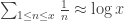for . (This formula has a delightful interpretation as an analytic formulation of the fundamental theorem of arithmetic.) Since neither side of the above formula makes sense when , Euler did the most logical thing possible and set anyway, to obtain

.

Taking logarithms, he then obtained

,

and expanding out all the logarithmic terms on the right as power series and regrouping, the right side becomes

.

Since all the terms except the first add up to something finite, they will not make a significant contribution in the limit, so Euler ignored them. (He could also have truncated after the first term when expanding the logarithms as power series, which would have had the same effect.) Hence, in the limit,

.

Naturally, that should be interpreted as

.

One can get rid of all the divergent series and weird expressions like by taking limits and being careful with error terms like a modern mathematician would do. But that wasn’t a necessary part of the culture in the 18^th century.

At this point, Euler stopped, but I don’t understand why. It is now possible to make an estimate for the number of primes up to , using a quick and easy computation. Since I’m a rebellious mathematician, I did the following computation on the front of an envelope.

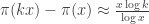
Let us try to estimate the number of primes between and , for some , and let us write for the number of primes up to . Then

,

where the explanation for the last term is that, if is not much bigger than 1, then each summand on the left is roughly . The goal is now to determine . We have

.

Expanding the logarithm using a power series and truncating after the first term, we obtain

.

Now, choosing and again taking the first term of the power series for the logarithm (that seems to be the name of the game today), we obtain

.

Now, summing over gives

(where I wrote 2 instead of 1 as the lower bound for the sum and integral to make them converge). And that’s one version of the prime number theorem. Nothing here would have caused Euler to break a sweat. But yet Gauss seems to have been the first one to conjecture the prime number theorem, and even he apparently did so on the basis of actually working out tables of primes and counting.

The Wallis Product

I had seen the Wallis product, but I did not know a derivation of it until a few weeks ago, when I discovered this gem when reading the wonderful book Sources in the Development of Mathematics by Ranjan Roy. I’m storing this example to use next time I teach calculus, as it requires nothing more than integration by parts.

Like in the case of many other such things in mathematics, I don’t know what the Wallis product actually is; I can only discover it by going through a derivation. So, I won’t give away the answer until we get there. But the goal is to write down an infinite product for .

In order to do this, we evaluate the integral . The first few are easy:

.

I can keep working out more of these, but now it’s time to tackle the general case, using integration by parts. We assume , and we compute , where and , so that

.

Solving for , we get . Now it’s easy to compute more of the ‘s:

,

and in general

.

Now, note that for any , , since whenever . Furthermore, since , this means that eventually and get very close together. So

,

or

.

(If we wanted, we could be more precise, and give two inequalities for , but it doesn’t add much value, in my opinion, to do that here.)

Taking the limit, we get

.

This is the Wallis product.

One interesting thing: Counting skew ternary trees

On Monday, I attended Don Knuth’s annual Christmas Tree Lecture, where he talks about the most interesting thing he has learned about trees in the past year. This year, he talked about ternary trees and planar graphs. Among other things, he showed us a beautiful theorem with a correspondingly beautiful proof, which I shall reproduce here.

A (nonempty) ternary tree is a tree consisting of a root node, and (possibly) several other nodes, so that each node has at most three children (denoted left, middle, and right). We draw ternary trees like this:

In this ternary tree, A is the root node, and it has a left child (B) and a right child (C), but no middle child. B has a left child (D) and a middle child (E), but no right child. C has a left child (F) and a middle child (G), but no right child. D has only a right child (H). Some nodes (E, F, G, and H) have no children.

If we have a ternary tree, we can assign ranks to the vertices, as follows: the root gets rank 0, and if a node has rank , then a left child (if there is one) will have rank , a middle child will have rank , and a right child will have rank . Hence, in the above tree, A and F have rank 0; B, E, and H have rank ; D has rank ; C and G have rank 1.

We call a ternary tree a skew ternary tree if all the ranks are nonnegative. The question we’ll answer is, what proportion of ternary trees with nodes are skew?

Whenever we have such a question and, there is only one correct way to start: calculate a few terms and look up the sequence on the Online Encyclopedia of Integer Sequences. Fortunately for me, after going to the talk, I was able to remember enough of the terms of the total number of ternary trees to find it without having to do any calculation: it is sequence A001764, and it begins 1, 1, 3, 12, 55, 273, 1428, 7752. It tells me that there are of them. This isn’t too surprising, since the famous Catalan numbers enumerate binary trees (see Richard Stanley’s Enumerative Combinatorics Volume 2, Exercise 6.19(c)).

Unfortunately, the skew trees are not represented on OEIS, but since I remember the theorem, I can calculate them easily: the sequence begins 1, 1, 2, 6, 22, 91, 408, 1938. The theorem is as follows:

Theorem. The ratio of the number of skew ternary trees with nodes to the number of total ternary trees with nodes is .

I think this is a rather remarkable theorem, because I don’t see any a priori reason to expect any nice relationship between these two numbers. On the other hand, perhaps it’s not so different from the classical Catalan situation: there are ways to get from to by taking unit steps either up or to the right, and ways of doing this without every going below the diagonal line .

Before moving on to the proof, I want to pose a question to think about while going through the proof: can a variation of this argument be used to write down a formula for the Catalan numbers? I don’t see it, but I’d love to hear it if you do!

In order to prove the theorem, we start by filling in all the potential children, so that every node has three children or phantom-children. In addition, all nodes except the root have parent nodes, so in order to make the root act more like the rest of them, let’s add a phantom-parent for the root. Let us now count the phantom nodes: each node has exactly four neighbors or phantom-neighbors, so there are a total of edge-germs emanating from all the genuine nodes, put together. There a total of edges between genuine nodes, and each one counts as two edge-germs, so there are a total of phantom edge-germs, or $2n+2$ phantom nodes.

Now, we start from the root and trace the outline of the entire tree. Since we are civilised mathematicians, of course we go counterclockwise. As we go, we write down a list of numbers, adding a new one every time we hit a genuine node. It doesn’t matter what number we start with, but Knuth chose , so I’ll follow his lead. Now, as we trace, we hit genuine nodes at various times. When we do, we either increase or decrease our running total by one. If we’ve just gone around a phantom node, then we increase the total by one, whereas if we have just come from a (different) genuine node, we decrease it by one.

Let’s see this in action with the example above. After we add the phantom nodes, we get the following diagram:

We start just before the phantom parent-node to node A with . Then we move around the phantom parent node. This increases the total by 1, to . Continuing along the outline, we next reach node B, which decreases our count to . Then we go on to node D, which decreases our count to , and so on. Here is a table with the first few values.

A	A	B	D	D	D	H	H	H	H
-2	-1	-2	-3	-2	-1	-2	-1	0	1

We can also represent this table in pictorial form, just by keeping track of where we are in the running total after each step. Here is the picture for the above graph.

It’s a bit easier to keep track of what’s going on if we overlay this picture on five horizontal lines (also known as a musical staff), so we can see immediately where we are:

Now it’s easy to see that we start at and end at in this case. But in fact, that’s always true: we pass phantom nodes and edges between genuine nodes. The former decrease the count by one, and the latter increase it by 1, so we have a net by tracing the entire tree. So, we always start at and end at .

The next observation is that the root of the tree shouldn’t be thought of as being fixed in place. Instead, we can pick a new node to be the root and let everything dangle from there. But we should be a little bit more precise on this point: it’s not quite the root node that we want to choose, but the parent phantom node of the root. Once we have done that, if we keep all the other edges in the right order, we obtain another ternary tree. We can do this with each phantom node, and so we obtain a total of different ternary trees in this way.

The next thing to work out is how the list of running totals changes when we choose a new parent phantom node. But this is not so hard: we see the same increases and decreases starting from some point, but then it must wrap around from the beginning at some point. For example, if we pick the new parent phantom node to be the right phantom child of F, we obtain the following chart (marked with the red rectangle):

So far, we haven’t said anything about what distinguishes skew trees from arbitrary ternary trees, but there is a very nice interpretation of them in terms of the counts: they are exactly the trees that never return to . With that observation in mind, the proof of the theorem is now quite easy: since each trace around the outline of the tree increases the count by 4, if we trace the outline of the tree many times, there will be several places where we encounter certain counts for the last time. These will certainly be before phantom nodes, rather than genuine nodes, since genuine nodes decrease the count. Those phantom nodes are exactly the phantom nodes that lead to skew ternary trees if we hang the tree from them. Since the count increases by 4 when we trace the outline once, there will be four such phantom nodes in each trace, out of a total of . Hence, the proportion of skew trees among any one such family is , and so the proportion of all ternary trees which are skew is also .

 

So, that’s the proof. Can this method be used to come up with a formula for the Catalan numbers as well? It seems as though this should be possible: in a path from to with right and up steps, there are a total of edges and vertices. We can add in the phantom neighbors to obtain phantom nodes. The goal would be to show that it is possible to hang the picture up from each one of the phantom nodes, so that each one leads to a suitable lattice lath, and of those, exactly 4 of them don’t go below the diagonal. But I don’t know how to do this, so I’d be interested to hear suggestions.

Exchange sacrifices galore

Last weekend, I played the BayAreaChess Thanksgiving tournament. My play was pretty bad, but my results (2 wins, 1 draw, 2 losses against all players rated a bit higher than I) were okay, and I hit a new rating high of 2050 after the tournament. This game, the most exciting but definitely not the best-played, features a total of three exchange sacrifices, followed by a sharp endgame culminating in a pawn race. All in all, it was an amusing if inaccurate game.

Simon Rubinstein-Salzedo (2037) vs. Julian Lin (2106)

1. e4 c5 2. Nf3 d6 3. d4 cxd4 4. Nxd4 Nf6 5. Nc3 a6 6. Be3 e5 7. Nb3 Be6 8. f3
Be7 9. Qd2 O-O 10. O-O-O Qc7 11. Kb1

Unfortunately, I don’t know my lines in the Najdorf as well as I should. The main move is 11. g4, but I was under the impression that white is supposed to wait until black plays Nbd7 to play g4. (At least, that was my rough heuristic.) But my move is okay as well.

11…Nbd7 12. Qf2

But I still didn’t play g4 immediately, because I wanted to stop black from playing Nb6 first.

12…Rfc8 13. g4 Qd8

Black is now planning to follow up with Rxc3. So, at this point I had to decide how to evaluate the position after the exchange sacrifice. I thought that if I could isolate some of black’s pieces on the kingside and out of trouble, then black would fail to get full compensation. So, I was willing to encourage the sacrifice.

14. g5 Nh5 15. Rg1

15…Rxc3!

Exchange sacrifice #1. I was pretty optimistic here, because the knight on h5 isn’t actively helping in the attack for the time being, and the e7 bishop also isn’t currently terribly useful.

16. bxc3 Qc7 17. Qd2

An interesting idea is to clarify matters on the kingside and give up the c-pawn with 17. Qh4. My idea was to give up the dark-squared bishop when the knight goes to b6 (since allowing it to get to a4 is unpleasant) and not worry too much when the other knight goes to f4.

17…Nb6 18. Bxb6

Unfortunately, the e3 bishop was doing double duty: stopping one knight from getting to b6, and the other from getting to f4. But I thought that allowing the knight to get to a4 would lead to very bad things for me.

18…Qxb6 19. Bd3 a5 20. Ka1 a4 21. Nc1 Qc5

This was a crafty move, and it took me a little while to understand what was going on: black threatens to play 22…Qa3.

22. Ne2

The idea is to meet 22…Qa3 with 23. c4 b5 24. Qc3

22…Bd8!

Another nice move, bringing the bishop into the game.

23. Rb1?

After 23. c4, black is a bit better, but white is in better shape than in the game.

23…Ba5

24. Rb4

Exchange sacrifice #2. I was originally planning to play 24. Rb5, but after 24…Qa3, white is simply lost. For example, 25. Rb2 Nf4, and c3 falls. So, this exchange sacrifice was forced.

24…Bxb4 25. cxb4 Qf2 26. Qe1 Qxf3

That was the best I could do: go down a pawn, but my structure is somewhat improved, and at least for the time being, black’s attack has been slowed. Objectively, though, I think my position is lost. So, the goal is to do the best I can setting up a fortress and not making any new weaknesses.

27. h4 Qe3 28. Qc1 Qb6

I was mildly surprised by this decision. Okay, black has some attacking chances still, but I expected that my opponent would prefer an endgame with a clear extra pawn. And, to be honest, I was hoping that he would trade queens, given that I have worked quite hard on endgames recently and thought I might hold, even if I didn’t really deserve to.

29. a3 Rc8 30. Rf1 g6 31. Qd2 Bg4!

Good idea: my bishop is relatively useless, being blocked in by my own pawns. (Capablanca’s rule: when you have a bishop, you should put your pawns on the opposite colored squares.)

32. Rd1 Bxe2 33. Bxe2 Nf4? 

This is what I expected, and it’s the most logical move, but 33…Ng3 simply wins another pawn. After this inaccuracy, I can put up some serious resistance.

34. Bg4! Rd8 35. c4

I had been counting on the strength of this pawn structure for some time. It’s no longer easy for black to break through, since d5 never works, b5 probably doesn’t work, a4 might be weak, and white might be able to play c5 in certain circumstances. At this point, I thought I had reasonable chances to hold.

35…Qc6 36. Qc2 Ra8 37. Rc1 b6

This attempt to get the rook back to the c-file was logical enough, but it’s not clear what the point is: I just keep my queen and rook on the c-file and shuffle my king, and how is black going to do anything?

38. Kb1 Kg7 39. Ka1 Ra7 40. Kb2 Ra8

So, he figured out that that idea wasn’t going to work. But what is happening next?

41. Ka1 Rh8

Yeah, that seems like a better plan. For some time, I had been thinking about playing h5 gxh5 Bf5, but now is my last chance to do it.

42. h5 gxh5 43. Bf5 h6 44. gxh6+ Kxh6? 45. Qh2?

A better move is 45. Rg2, trapping the king on the h-file. The idea is that, while there are several things black wants to do, it’s hard to do all of them: if the queen goes to a8 to prepare Rg8 and a rook trade, then I have Qd2, hitting the d-pawn. If the queen stays on c6, then I can play Qh2 and Qg3 (sacrificing the c-pawn), setting up threats on the g-file.

45…Rg8 46. Qh4 Rg5 47. Qh2 Rg2 48. Qh4 Rg5 49. Qh2

I’m not going to complain about a draw here. But he won’t have any of that.

49…Rxf5?

Exchange sacrifice #3. This is not the best way to continue though: 49…Rg2 50. Qh4 Kg7 51. Rc3 Ne2 is completely winning for black. His move might be winning too, but it gives me more chances. One point to notice is that I’m not seriously threatening anything: he could just take some time to put his king in a safer spot before continuing, and I wouldn’t be able to do anything in the meantime.

50. exf5 Qf3 51. Qa2 Qe3 52. Rd1 Qc3+?

It’s better to win the f-pawn first with 52…Kg5 and then push the h-pawn. At the very least, it buys time for a pawn race, which, as we shall see, is very important later in the game.

53. Kb1 Nd3?

It’s probably still a draw with best play, but now white has most of the winning chances.

54. Qd2+ Qxd2 55. Rxd2 e4 56. Re2 Kg5 57. Rxe4 Kxf5 58. Rd4 Ne5

I didn’t know what was going on here during the game, but I knew what I had to do: activate my queenside pawns before black’s kingside pawns get too dangerous. First plan of action: defend my c-pawn with my king so that I can win the d- and b-pawns, and try to do so quickly enough that I can still stop the black pawns on the kingside. But will it work?

59. Kc2 Kg5 60. Kc3

So far, we have stayed in drawing territory. But now black has a decision to make: which pawn to push? Is it better to have two relatively advanced pawns, or one very advanced pawn?

60…f5?

It’s sometimes hard to figure out what to do when you have two passed pawns, but here’s a pretty good heuristic: bet everything on the one that’s the most advanced. This heuristic would lead to the correct move in the case: 60…h4, which draws. For example 61. Rxd6 h3 62. Rd1 Kf4 63. Kd4 h2 64. Kd5 Ng4 65. Rh1 Ne3+ 66. Kc6 Kg3 67. c5 bxc5 68. b5 Nc4 69. Kxc5 Ne5, and black can stop the b-pawn with the knight, so the game should end in a draw.

61. Rxd6 h4 62. Kd4?

In turn, I’m not sure what I missed, but 62. Rxb6 h3 63. Rd6 h2 64. Rd1 is pretty clearly winning for white. I guess the pressure of a long game was taking a toll on both of us by this point.

62…Ng4?

Better is 62…Nf3+!, because there are too many forks lurking.

63. c5!?

This is probably winning, and it’s very exciting to go into a pawn race and get some new queens on the board, but 63. Rxb6 h3 64. Re6 is a much easier and less stressful way to win.

63…h3 64. cxb6

Not 64. c6?? h2 65. c7 h1Q 66. c8Q Qd1+ 67. Kc4 Qc1+, winning the queen.

64…h2 65. b7 h1=Q 66. b8=Q

I evaluated this as probably winning, but I’m not sure, and anyway with limited time remaining, I didn’t know what would happen. After the expected 66…Qc1, it’s still a tough game. Fortunately for me, though, he quickly went astray.

66…Qe4+

Maybe this isn’t a horrible move objectively, but it puts the queen in a vulnerable spot, and that’s not a smart thing to do in a complicated position after 5 hours with little time remaining.

67. Kc5 Ne5??

But this loses instantly.

68. Qd8+ Kg4 69. Rd4 1-0

My opponent deserves a lot of credit for extracting a lot from an exchange sacrifice that I didn’t initially believe in (Rxc3). I knew that in the Dragon, Rxc3 always works, but I was more skeptical about its strength in the Najdorf. I guess now I know better to allow it in the future. I also need to know my lines in the Najdorf better if I’m going to continue to play open Sicilians: it’s simply irresponsible to enter into such sharp lines without being well-prepared. (In fact, all three of my white games in this tournament featured the Najdorf. It was only in the third game that I responded relatively well.) Probably I would see the most benefit in my chess ability if I were to work on my openings and learn some systems properly. But how do I do that in the most effective way possible? I could memorize a bunch of lines blindly à la Moonwalking with Einstein using memory palaces or something similar, but I have fundamental objections to using such techniques, since they cause people to remember things for all the same reasons. Anyway, I’m constantly telling my students not to memorize things. Alternatively, I could play through a bunch of games and hope that the lines stick, but usually they don’t, as there is so much to learn. So, how do you learn openings?

One interesting thing: Average polynomial time algorithms

The most celebrated problem in theoretical computer science is undoubtedly the P vs. NP problem. Let me explain what it is asking. (If you already know this, feel free to skip the next few paragraphs.) Suppose we have a general type of problem that we wish to solve. (Think of something like determining if a number is prime, or factoring it.) There are many instances of such a problem. (For example, there are lots of numbers out there, and we could ask for each number whether or not it is prime.) Now, suppose we have a computer program that solves this type of problem: it runs for a while, and eventually tells us the answer. The amount of time it takes to run depends on the complexity of the specific problem we give it: for example, we should expect it to take longer to determine whether a very large number is prime than it would take for a small number, although there are some exceptions. (It would be very fast to say that a large number is composite if it is even, for instance.)

For the most part, then, the amount of time it takes to run the program depends on how complicated the particular instance of the problem is. We’ll measure that in terms of the number of characters needed to enter it. So, we can ask how long it takes to determine if an -digit number is prime, for example. (Answer: not very long, surprisingly.)

Normally, we aren’t particularly interested in exactly how long it takes to run in terms of number of seconds, because that changes from one computer to another. Instead, we’re interested in how the length of time grows as the length of the input grows. We say that a program runs in polynomial time if there is some polynomial so that the amount of time to solve any instance of the problem with an input of length is at most . Observe that this notion does not depend on the speed of the computer; for instance, if we switch to a computer that runs half as fast, that’s equivalent to multiplying by 2. We call a problem a P problem if it has an algorithm that solves it in polynomial time.

Now, let us consider the notion of NP, which stands for nondeterministic polynomial time. What this means is that, if I magically tell you the answer to a problem (but I might be lying to you), you can check whether I’m telling you the truth in polynomial time. A classic example of this is factoring. If I ask you to factor 51445627, you are unlikely to be able to do that quickly (although there are some very clever algorithms for doing it). But if I tell you that the prime factors are 5689 and 9043, then you can check this quickly, in polynomial time in the length of the original number. Note that all P problems are also NP problems: if you can solve the problem on your own in polynomial time, you can still solve it in polynomial time if I tell you the answer, for example by ignoring my answer.

The P vs. NP problem asks if P = NP. That is, can every problem that can be checked in polynomial time also be solved in polynomial time? Most people believe the answer to be no, but we have made little progress toward a proof.

Note that the property of being in P depends on all instances of the problem. However, computer scientists are a bit different from mathematicians: they don’t usually need to prove things; they just want to get right answers. (Probably not all of them, but that’s my view of it from a mathematician’s world.) So, might it be that there problems that can’t always be solved in polynomial time, but usually can?

This is the subject of Russell Impagliazzo’s very nice survey paper “A Personal View of Average-Case Complexity.” He rather amusingly frames the problem in terms of the famous story about a very young Gauss being asked to sum the numbers from 1 to 100, and the teacher’s subsequent attempts to humiliate Gauss in revenge for his quick solution. (Note: I don’t do that to my students. In fact, I like it when they are clever.)

In it, he includes a definition for an average polynomial time algorithm, which essentially means that if we were to choose a random instance of the problem, we would expect to be able to solve it in polynomial time. But before we can make that more precise, it is necessary to explain what we mean by a random instance of the problem. In order to do that, it makes sense at first to restrict to a given input size . In order to select a random instance of a problem of size , we need to put a probability distribution on the instances of the problem of length . Then, intuitively, to say that an algorithm is an average polynomial time algorithm is to say that there is a polynomial so that the algorithm solves nearly all instances of the problem of length , chosen according to , in time at most , and the “exceptional” cases get increasingly rare as gets larger. (The real definition is more precise, but this captures the essence of it.)

Now, one might ask whether there are any problems for which there exist average polynomial time algorithms but not polynomial time algorithms. Since we don’t know whether P = NP or not, it’s hard to be sure, but one problem that is very strongly believed not to be a P problem is the Hamiltonian path problem. Let us explain what it says.

A path in a graph is a sequence of edges so that each edge (other than the first) starts where the previous one ended. (So that we can imagine walking on it if we were on the graph.) A path is called a Hamiltonian path if it goes through each vertex once, without any repetitions.

The Hamiltonian path problem asks if, given a graph, we can determine whether there is a Hamiltonian path. This problem is definitely an NP problem: if someone tells us that there is a Hamiltonian path and tells us what it is, then we can quickly check whether it actually is. (However, if someone tells us that there is no Hamiltonian path, it is not clear how we would verify that quickly, and indeed we expect not to be able to do so.)

It is widely believed that the Hamiltonian path problem is not a P problem; in fact, if it were, then we would also have P = NP, since it is possible to convert any NP problem quickly into a Hamiltonian path problem.

So, we believe that we can’t solve the Hamiltonian path problem quickly in general. But what about for most cases?

In order for that question to make sense, we need to put a probability distribution on graphs with vertices, so that we can sample them. One way of doing that is with the Erdős–Rényi model that I discussed last week: we pick a random graph by saying that any two of its vertices will be connected with probability , independently of all the other pairs.

So, let’s fix a and let vary. Then, it turns out that there is an algorithm that can determine whether a graph has a Hamiltonian path in almost polynomial time. The algorithm is given in detail in Yuri Gurevich and Saharon Shelah’s paper “Expected Computation Time for Hamiltonian Path Problem,” but I’ll sketch the basic idea, which is very simple. (What they do is somewhat more subtle, but here’s my personalized version of it, which probably doesn’t actually work very well.) It runs in three steps:

1. Choose a potential starting point and a potential ending point. (There are only a polynomial number of pairs to choose, so we can run through all such pairs in polynomial time.) Try to make a Hamiltonian path by making a path from the starting point that’s as long as possible, just by trying to add one vertex at a time. Once we get into trouble, do the same thing starting with the ending point. Try to make minor modifications to splice these two pieces together.
2. If that doesn’t work, try to show there is no Hamiltonian path. To do this, identify troublesome vertices: the ones that have relatively small degree. See if there is a contradiction involving these problem vertices.
3. If that doesn’t work, simply check every possible path and see if it gives a Hamiltonian path.

Steps 1 and 2 can be done in polynomial time; it is only step 3 that can’t. But it turns out that we won’t reach step 3 very often, because most of the time the algorithm will have finished after step 1 or 2.

Okay, so it’s an example, although I don’t find it particularly satisfying: as gets large, almost all graphs chosen in this way have Hamiltonian paths, since they have so many edges! I’d be very likely to find one in Step 1, which just tries things at random. Thus, I could make an algorithm that says there is always a Hamiltonian path, and it will run very quickly and only very rarely be wrong.

So, I am curious to know whether there are more interesting examples of problems with average polynomial time algorithms but that are not expected to have worse-case polynomial time algorithms.

One interesting thing: Erdős–Rényi random graphs

I’ve been thinking a lot about random graphs this week, so it is appropriate for my post this week to be about them. One of the most important models of random graphs is the Erdős–Rényi model. Here is the construction: we fix some parameter with , and we choose some positive integer . Then, we draw vertices. Between each pair of vertices, we put an edge there with probability , independently of all the other pairs. I’ve been thinking about problems relating to evolutionary dynamics on such graphs, but I won’t describe that today. (Maybe I will at some point, when I understand them better.)

Instead, I just want to talk about the graphs themselves, since there are a lot of questions one can ask about the structure of them. What do they look like? In particular, are they likely to be connected?

The answer is that it depends on how large is relative to . There is a phase change at . In fact, we have the following theorem (which is not quite the best possible):

Theorem (Erdős–Rényi). For any , we have the following: 

1. If , then the probability that the graph is connected goes to 1, as goes to infinity.
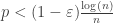2. If , then the probability that the graph is connected goes to 0, as goes to infinity.

I’m not going to give a proof here, but a proof can be found on this MathOverflow page.

But what happens when the graph is disconnected? To what extent does it fail to be connected? There is a very nice answer to this question as well:

Theorem. Suppose that is a constant. Then:

1. If , then with high probability all the connected components are small: they have size .
2. If , then with high probability there is exactly one large connected component, of size , for some number , and the rest of the connected components have size .

The large component when is called, suitably, the Giant Component. A proof can be find here.

There is a lot more than one can say about the Erdős–Rényi model for random graphs, but this will be enough for now.

One Interesting Thing: The preponderance of 2-groups among finite groups

This is a preliminary discussion of my knowledge about 2-groups. There are still many questions I have, and I would appreciate any insights.

When we first learn about group theory, we learn some theorems about how to decompose finite groups, most notably the Sylow theorems, which tell us (roughly) how to decompose groups based on their maximal -power subgroups. So, we might expect that for random finite groups, we can obtain a lot of information about them by analyzing what happens at each prime factor of the order.

And indeed, groups that appear “in nature” tend to have several prime factors, and their Sylow subgroups are typically interesting objects in their own right.  However, if we count groups not by their occurrences in nature but simply by their orders, then we see something very different: most finite groups are 2-groups: their order is a power of 2, so there is no information to be obtained by looking at other primes.

I was surprised at first to learn that the vast majority of groups are 2-groups: for example, there are 49,910,529,484 group of order up to 2000, and of those, 49,487,365,422, or more than 99%, have order . And the proportion of groups with 2-power order will only increase to 1 as we go further.

I don’t really understand why this is true (I have only barely skimmed the relevant papers, such as Eick and O’Brien’s “Enumerating -groups” and Besche, Eick, and O’Brien’s “The groups of order at most 2000”), but here is my vague intuition. The Jordan-Hölder theorem tells us that we can assemble groups out of simple groups. Now, it is likely possible to glue two large simple groups together in quite a few ways, whereas there are fewer ways of assembling two small simple groups together. However, more relevant than the size of the pieces is the number of pieces: a Jordan-Hölder series for a group of order 1024 will contain ten factors, each isomorphic to . As we all learned when we were very young and trying to assemble jigsaw puzzles, there are lots of ways of putting together many small pieces, but there are not so many ways of putting together a few large pieces. And this is just as true of groups as it is of jigsaw puzzles.

But there’s a problem with this analysis: there are way more groups with order 1024 than there are with , even though they contain the same number of factors in their composition series. In fact, there are 408,641,062 of order 1536, which is only roughly 40 times as many as there are groups of order (as opposed to nearly 5000 times for 1024). I would like to understand this discrepancy, but I’m not there yet.

One obstacle to understanding this point for me is that there isn’t such a discrepancy for groups of order versus when is small: for example, when and , there are 14 groups of order 16, 15 of order 24, 14 of order 40, 13 of order 56, and so forth. Similarly, when , there are 51 groups of order 32, 52 of order 48, 52 of order 80, and 43 of order 112. Since I don’t know any exciting examples of groups of order for large, it’s hard for me to gain intuition about what’s going on here.

There are lots of things to look into in the future, such as reading the papers by Besche and Eick. Perhaps I’ll report on them in the future.

One Interesting Thing: Homomorphic Encryption

I plan to start writing about one interesting thing I learn each week. This will serve two purposes: forcing me to think about interesting things, and also forcing me to write. Here is the first installment in the series.

Suppose I have a lot of computation I need to do, based on some initial data. (I sometimes find myself in this situation, having to calculate tables of number fields or something else of this flavor.) I could buy a supercomputer to do it for me, but then maybe I don’t need to these big computations very frequently, so it would be an expensive investment to buy a supercomputer for only occasional use. So instead, I decide to rent computing power from someone else’s supercomputer, so that I can upload my program and data to that other supercomputer.

Oh, but there’s a problem: my data are rather sensitive (so I’m probably not just computing tables of number fields), and I don’t know if the owner of the supercomputer is trustworthy or not. So I have to encrypt my data.

But now I have another problem: I have to do computations with my data, but they are encrypted. So, how do I do computations on encrypted data?

Let’s illustrate the problem with a simple example. Suppose my data consist of a string of letters. I encrypt them with a substitution cipher, replacing each letter with some other letter. So maybe I replace all instance of the letter “A” with “Q,” all instances of “B” with “D,” and so forth, making sure not to have any duplicates. Suppose I wish to increment the third letter of my string by 2, so if it was originally an “A,” then it should become a “C,” and if it was originally an “H,” then it should become a “J,” and so forth. How do I do it?

Well, if I have access to the original string, then it’s easy: just change that character. But what if I only have the encrypted version? I look at the string, and I see that the third letter is a “U.” But it wasn’t originally a “U”; that’s just the encrypted version of some letter. So, I don’t know how to increment it.

So, in order to do this increment procedure, I first have to decrypt the message. If I want this to be done on the supercomputer, then I need to provide it with the substitution key. But if I’m going to do that, then why did I bother encrypting it in the first place? My data is no longer securely encrypted. Alternatively, I could send the string back to my own computer, where I could do the process safely, and then encrypt it again and send it back to the supercomputer. But then what is the point of renting supercomputer time if I’m going to have to send the data back to my own computer whenever I want to do a computation?

In order to solve these problems, I need to encrypt my data in such a way that it is still possible to perform computations on it even when it is encrypted. To see how I might do this, let us return to the letter substitution example. If instead of having some weird rule about how to substitute letters I use a Caesar cipher, where my encryption is simply to push every letter forward by five positions (so that “A” becomes “F,” “B” becomes “G,” and so forth), then I can ask the supercomputer to increment the third letter by two positions even in its encrypted form, since incrementing the encrypted version by two also increments the unencrypted version by two.

This is a simple example of homomorphic encryption. Of course, the Caesar cipher is a terrible way of encrypting data, as it is trivial to decrypt. But some trickier encryption schemes like the Vigenère cipher also have the same property. They still aren’t secure, but we’re making small amounts of progress.

Unfortunately, my scope is still very limited here: I can increment some characters by fixed amounts, but I can’t perform other string operations. For example, I can’t replace the third character with a “T.” And if I’m using a Vigenère cipher, then I can’t reverse the string either. I want to be able to do more interesting operations with the ciphertext. Can I find an encryption method that will let me do everything I want just by acting on the ciphertext?

This is the question that homomorphic encryption answers. I won’t explain how to do the full version of it, but here’s a limited version, that can only deal with plaintext strings that are either 0 or 1 (so, two possible choices). Clearly, that isn’t sufficient for all our cryptographic needs, but it will serve to illustrate how some of this stuff works anyway.

Let be a binary digit, so either 0 or 1. To encrypt it, we choose integers . I’ll explain how they are to be related (i.e. how big they are) later. To encrypt , I first pick a key , which will be an odd, -digit binary number (so the last digit is a 1). Now, let be a random -digit number whose last digit is (i.e. ). Also, pick a random -digit binary number . Encrypt as .

Decrypting is easy if we know : , where means the unique integer from 0 to congruent to modulo .

Craig Gentry, in his paper “Computing Arbitrary Functions of Encrypted Data” from which I learned most of this material, suggests choosing a parameter and then setting , , and . These choices don’t matter too much, and indeed I might suggest making a little larger relative to , but they are suggestive of how large they need to be relative to each other.

Now, why is this encryption scheme homomorphic? If I have two plaintext messages and , with ciphertexts and , respectively, then and are encrypted versions of and , respectively. (Note that I say “encrypted versions” rather than “the encrypted versions,” because there are many ways to encrypt the same message due to the random choices of and .)

However, we have to be a bit careful here, because the underlying point in this encryption scheme is that is close to being a multiple of and the relevant part of it (namely ) is small relative to . But if we do lots of operations, then the bit can get ever larger, so that it is no longer small relative to .

The conclusion is that this setup allows us to perform operations on a ciphertext a few times, but after that, we cannot reliably decrypt it into what we were supposed to get.

The Gentry paper explains how we can fix this problem into a fully homomorphic encyrption scheme, so that we can perform as many operations as we want. His paper is refreshingly readable, and he prefaces each of his technical remarks by an allegory of a jewelry store in which the owner (named Alice, appropriately enough for a paper on cryptography) does not trust her workers not to steal expensive jewels if they can get their hands on them.

Also helpful is this blog post by Craig Stuntz, called “What is Homomorphic Encryption, and Why Should I Care?” I recommend reading that before the Gentry paper for an explanation of the background of homomorphic encryption.

An experiment in imbalances

Ordinarily, when I play chess, I favor relatively balanced positions, in which the result of the game is more likely to hinge on positional ideas, rather than tactics. Hence, I do not sacrifice material often, unless I have calculated that doing so is guaranteed to work. However, this past weekend, I played a game in which I was inspired to play more freely, sacrificing material for evident compensation, but no clear win.

 

Simone Liao (2202) vs. Simon Rubinstein-Salzedo (2026)

My opponent is yet another of the endless string of very strong kids to play chess in the Bay Area. It’s actually a rather unusual occurrence to play against someone who has graduated from high school around here, even in the master section of a tournament. This particular kid has the distinction of being the top woman under age 21 in the country, despite being only 14!

1. e4 e6 2. d4 d5 3. Nc3 Bb4 4. e5 c5 5. a3 Bxc3+ 6. bxc3 Ne7 7. Qg4 Qc7 8. Qxg7 Rg8 9. Qxh7 cxd4 10. Ne2 Nbc6 11. f4 dxc3 12. Qd3

Up to here, everything is completely standard, except that perhaps 11…Bd7 is slightly more common than 11…dxc3. With 12…Bd7, we would transpose back into the most common line, but I wanted to play something different.

12…d4

I was still well within my book knowledge at this point, but my opponent started to think for the first time after this move. Before this, we had each only taken a few seconds to play all of our moves. The most testing line is 13. Nxd4, but she opted for what I consider to be a less dangerous variation.

13. Ng3

This is still a known move, but I forgot what the textbook response is. Fortunately, it isn’t very hard to find: white wants to put her knight on either d6 or f6 after Ne4 (or Nh5), so I have to make sure that that isn’t particularly dangerous.

13…Bd7 14. Ne4 O-O-O

White can win a pawn with 15. Nd6+ Kb8 16. Rb1 b6 17. Nxf7, but after 17…Rdf8 18. Nd6 Nf5, it may well be black who benefits more from the loss of the pawn, due to the files available for the rooks. Thus, it makes sense to play something else. In my understanding of this opening, white suffers a bit by having an exposed king and somewhat awkward piece play, but the compensation is a passed h-pawn that can become dangerous quickly if black is slow to react. Therefore, my opponent’s next move seems very reasonable.

15. h4

Okay, so white’s plan is clear. As for black’s plan, well, nothing makes a French player happier than acquiring mobility for the central pawns. One way of obtaining that is by playing f6 and trying to trade them off. However, I favored a more dramatic way of accomplishing this task: blowing the center open with a piece sacrifice. I didn’t want to play 15…Nxe5 immediately though, because I was concerned about 16. Qxd4. It turns out that black is doing fine, but I preferred to defend the d4-pawn first and then see what would happen.

15…Nf5 16. Rh3

16…Nxe5!?

Definitely not the way I usually play chess, but it felt like such a logical thing to do. Her king is stuck in the center, so I have an attack that isn’t going away any time soon, and there isn’t any clear way for white to clarify the position. I believe that I get full compensation for the knight, but no more. (I’m certainly not winning, which is reasonable, because white hasn’t done anything wrong.)

The main line I calculated before playing 16…Nxe5 was 17. fxe5 Qxe5 18. Qe2 Bc6 19. Nf2, after which I get my material back. But of course 19. Nf2 isn’t the strongest line.

17. fxe5 Qxe5 18. Qe2 Bc6 19. Ng5!

Definitely the right move. Before I played 18…Bc6, I realized that there were plenty of reasonable options other than Nf2, and I had to work out that in particular 19. Nxc3? loses (to 19…Qa5!). I also had to work out what happened after Ng5, calculating the line played through move 23.

19…Qxe2+ 20. Bxe2

20. Kxe2 f6 and now 21. Nxe6? is impossible due to 21…Rde8, winning the knight, with a big edge for black.

20…f6 21. Nxe6 Rde8 22. Nf4

And now I have two ways of recovering some material: 22…Bxg2 and 22…Ng3. I chose wrong, unfortunately.

22…Ng3 23. Rxg3

Forced. Black threatens 23…Nxe2 24. Nxe2 Rxg2. And after 23. Rh2, 23…Bb5 wins (although not my planned 23…Rxe2+? 24. Nxe2 Re8 25. Kf2 Nxe2 26. h5, and white is better).

23…Rxg3 24. Kf2 Reg8 25. Bf1

Now is a good time to take stock of the position. I felt that I was the one playing for a win here, although it’s not necessarily clear what to do. My logic, though, is that white’s pieces are rather awkwardly placed. She has to keep a bunch of pieces defending g2, and in the meantime it’s not so easy to get the queenside pieces into the game. However, it’s not so easy for me to improve my position and increase pressure. So, I decided to eliminate Ne6 possibilities.

25…Kd7? 26. h5 Be4 27. Ra2?

This seems logical enough, and it’s what I expected, but actually 27. Rb1! is much stronger, and white is doing very well. Because of this possibility, it was better to switch my 25th and 26th moves, as 25…Be4 more or less forces 26. Ra2. (The computer initially considers 26. h5 a viable option for tactical reasons, but at deeper levels of analysis, it turns out not to work very well.)

27…R3g4 28. Bd3 f5

28…Bxd3 is actually better, since white quickly gets in zugzwang: 29. cxd3 Rh4 30. Rc2 Re8, and there is no way to save the h5-pawn. However, white can still draw with 31. Ne2 Rxh5 32. Nxd4 Rd5 33. Be3 Rde5 34. Bc1 Rd5, repeating moves. During the game, though, I thought I would do well to encourage a bishop trade if doing so would allow me to strengthen my central pawn mass. After 29. Bxe4 fxe4, the central pawns are rather dangerous.

29. Bf1 Kd6 30. Ng6

30…R8xg6!?

I felt that playing this move was the height of frivolity, as there is really no need to sacrifice the exchange here. However, I couldn’t imagine that I might be worse after doing so, and the sacrifice eliminates one of white’s main sources of play. (Note how most of the white pieces are rather tied down.)

31. hxg6 Rxg6 32. Bf4+ Kc5 33. a4

This was a move I was hoping to be able to prevent, but then there it was. I was about to play 33…a5, but then I noticed something interesting.

33…Rb6!

With the threat of 34…Rb2. There is only one way to defend.

34. Bc1 Rb1 35. Ba3+ Kb6

And now I threaten 36…Bd5. Again there is only one defense (although she can throw in 36. a5+ first).

36. Bc4 Rd1

And now white loses at least a pawn.

37. a5+ Kc6

Not 37…Kxa5?? 38. Bc5#, but typically players at this level don’t do things quite that stupid.

38. Bb3 f4

The g-pawn will still be available later, so I wanted to prevent her from getting her king activated.

39. Be7 Rd2+ 40. Kf1?

So far, she has defended fairly well, and after 40. Ke1 Rxg2 41. Bf6, the game is close to equal. One possible line is 41…Bd5 42. Ra4 Bxb3 43. cxb3 c2 44. Rc4+ Kd5 45. Bxd4 c1Q+ 46. Rxc1 Kxd4, which white can hold easily. But after 40. Kf1, black is winning.

40…Bxg2+ 41. Kg1 Bd5 42. Ba4+ Kc7 43. Ra1 Rg2+ 44. Kf1 f3

Threatening 45…Bc4+, so white has to abandon defense of the c-pawn.

45. Bb5 Rxc2 46. Bf6 Rd2?!

The zwischenzug 46…a6! wins immediately: 47. Be5+ Kd8! (not Kc8, after which white gets an extra check on a light square and can therefore put up stiffer resistance) 48. Bd3 Rd2 49. Bf6+ Kc7, and the light squared bishop cannot move off the diagonal and must therefore be sacrificed.

After 46…Rd2, black is still winning, but I started losing the thread, as the bishops became increasingly active.

47. Bg5 Rb2 48. Bd3 Kc6 49. Bc1 Rh2 50. Kg1 Rg2+ 51. Kf1 Kc7?

I wanted to bring my bishop around to h3 without having something nasty happen on e4, but this is the wrong way to play. Instead, 51…f2! with the idea of running white out of moves wins comfortably. For example, 52. Rb1 c2 53. Ra1 (53. Rb2 Rg1+ 54. Kxf2 Rxc1 55. Bxc2 Ra1, and winning with three extra pawns is trivial) Rh2 54. Be2 Be6 55. Bf3+ Kc5 56. Bg2 Bd5 57. Ba3+ Kc4 58. Bxd5+ Kxd5, and the pawns win.

After this, there are still some chances for black, but we were reaching the time trouble stage after nearly five hours of play, and so there wasn’t sufficient time to make sure that our moves made much sense.

52. Rb1 a6 53. Bf4+ Kd7 54. Rb6 Bc6 55. Rb4 Ra2 56. Rxd4+ Ke7 57. Bd6+ Kf6 58. Rf4+ Kg5 59. Rf5+ Kg4 60. Rf4+ Kg5 61. Rf5+ Kg4 1/2-1/2

Neither one of us knew during the game whether this position was equal, or if not, who was better, but with 2 minutes each, we were both happy not to do anything really stupid and split the point.

I found it quite freeing to sacrifice material in this game. It has been several years at least since I last sacrificed material for any reason other than a forcing line or out of desperation in a bad position, but it might be worth trying it out again in the future.

I’d say that the opening line I played in this game was a great success, because my opponent (with the white pieces) did nothing wrong in the opening, but I was still able to sacrifice a piece and get full compensation for it. From a philosophical point of view, it’s hard for me to understand how that is possible, but perhaps the philosophy is irrelevant, and I simply ought to enjoy the games I can get out of it.